The Dataset
Our goal for this experiment is to determine which Arabidopsis thaliana genes respond to nitrate. The dataset is a simple experiment where RNA is extracted from roots of independent plants and then sequenced. Two plants were treated with the control (KCl) and two samples were treated with Nitrate (KNO3).
The sequences were processed to remove all low quality sequences, trim all low quality nucleotides, and finally aligned against the Arabidopsis genome using TopHat. Our analysis starts from here.
We have been provided the following files:
- 4 Bam files – An alignment file, one for each sample
- Arabidopsis.gtf file – which contains information about the genes in Arabidopsis and where they are located in the genome.
- Experiment design – a comma separated file containing meta data.
- Gene description – Description about the function of the genes in Arabidopsis.
Note: If one of the R packages is not loaded, you have to install it from Bioconductor
source("http://bioconductor.org/biocLite.R")
biocLite("Rsamtools")
biocLite("GenomicFeatures")
biocLite("GenomicAlignments")
biocLite("DESeq")
The Data Files
The Alignment Files
The alignment files are in bam format. This files will not be loaded into R, but rather simply pointed to by a reference/variable. The alignment files provided are about 15x smaller compared to an average RNA-seq sample run today. Also there will be triplicates of 3 or more different conditions resulting in much more than 4 sample. So you can imagine the amount of space and memory R would need if all that data was stored in the workspace.
To do point to the bam files we will use Rsamtools
library(Rsamtools)
## Loading required package: S4Vectors

## Warning: package 'S4Vectors' was built under R version 3.2.3

## Loading required package: stats4

## Loading required package: BiocGenerics

## Loading required package: parallel

##
## Attaching package: 'BiocGenerics'

## The following objects are masked from 'package:parallel':
##
## clusterApply, clusterApplyLB, clusterCall, clusterEvalQ,
## clusterExport, clusterMap, parApply, parCapply, parLapply,
## parLapplyLB, parRapply, parSapply, parSapplyLB

## The following objects are masked from 'package:stats':
##
## IQR, mad, xtabs

## The following objects are masked from 'package:base':
##
## anyDuplicated, append, as.data.frame, as.vector, cbind,
## colnames, do.call, duplicated, eval, evalq, Filter, Find, get,
## grep, grepl, intersect, is.unsorted, lapply, lengths, Map,
## mapply, match, mget, order, paste, pmax, pmax.int, pmin,
## pmin.int, Position, rank, rbind, Reduce, rownames, sapply,
## setdiff, sort, table, tapply, union, unique, unlist, unsplit

## Loading required package: IRanges

## Warning: package 'IRanges' was built under R version 3.2.3

## Loading required package: GenomeInfoDb

## Warning: package 'GenomeInfoDb' was built under R version 3.2.3

## Loading required package: GenomicRanges

## Warning: package 'GenomicRanges' was built under R version 3.2.3

## Loading required package: XVector

## Loading required package: Biostrings

## Warning: package 'Biostrings' was built under R version 3.2.3
(bamfiles = BamFileList(dir(pattern=".bam")))
## BamFileList of length 4
## names(4): KCL1_dedup_sorted.bam ... NO32_dedup_sorted.bam
The Annotation File
GTF file is very similar to a GFF file. Their purpose is to store the location of genome features, such as genes, exons, and CDS. It is a tab delimited flat file which looks something like this.
## reference source feature start stop score strand phase
## 1 Chr1 TAIR10 exon 3631 3913 . + .
## 2 Chr1 TAIR10 exon 3996 4276 . + .
## 3 Chr1 TAIR10 exon 4486 4605 . + .
## 4 Chr1 TAIR10 exon 4706 5095 . + .
## 5 Chr1 TAIR10 exon 5174 5326 . + .
## 6 Chr1 TAIR10 exon 5439 5899 . + .
## annotation
## 1 transcript_id AT1G01010.1; gene_id AT1G01010; gene_name AT1G01010;
## 2 transcript_id AT1G01010.1; gene_id AT1G01010; gene_name AT1G01010;
## 3 transcript_id AT1G01010.1; gene_id AT1G01010; gene_name AT1G01010;
## 4 transcript_id AT1G01010.1; gene_id AT1G01010; gene_name AT1G01010;
## 5 transcript_id AT1G01010.1; gene_id AT1G01010; gene_name AT1G01010;
## 6 transcript_id AT1G01010.1; gene_id AT1G01010; gene_name AT1G01010;
We will load the GTF file using GenomicFeatures and group the exons based on the gene annotation.
library(GenomicFeatures)
## Warning: package 'GenomicFeatures' was built under R version 3.2.3

## Loading required package: AnnotationDbi

## Warning: package 'AnnotationDbi' was built under R version 3.2.3

## Loading required package: Biobase

## Welcome to Bioconductor
##
## Vignettes contain introductory material; view with
## 'browseVignettes()'. To cite Bioconductor, see
## 'citation("Biobase")', and for packages 'citation("pkgname")'.
txdb <- makeTxDbFromGFF("Arabidopsis.gtf", format="gtf")
## Import genomic features from the file as a GRanges object ...

## OK

## Prepare the 'metadata' data frame ...

## OK

## Make the TxDb object ...

## OK
(ebg <- exonsBy(txdb, by="gene"))
## GRangesList object of length 33610:
## $AT1G01010
## GRanges object with 6 ranges and 2 metadata columns:
## seqnames ranges strand | exon_id exon_name
## |
## [1] Chr1 [3631, 3913] + | 1
## [2] Chr1 [3996, 4276] + | 2
## [3] Chr1 [4486, 4605] + | 3
## [4] Chr1 [4706, 5095] + | 4
## [5] Chr1 [5174, 5326] + | 5
## [6] Chr1 [5439, 5899] + | 6
##
## $AT1G01020
## GRanges object with 12 ranges and 2 metadata columns:
## seqnames ranges strand | exon_id exon_name
## [1] Chr1 [5928, 6263] - | 21880
## [2] Chr1 [6437, 7069] - | 21881
## [3] Chr1 [6790, 7069] - | 21882
## [4] Chr1 [7157, 7232] - | 21883
## [5] Chr1 [7157, 7450] - | 21884
## ... ... ... ... ... ... ...
## [8] Chr1 [7762, 7835] - | 21887
## [9] Chr1 [7942, 7987] - | 21888
## [10] Chr1 [8236, 8325] - | 21889
## [11] Chr1 [8417, 8464] - | 21890
## [12] Chr1 [8571, 8737] - | 21891
##
## $AT1G01030
## GRanges object with 2 ranges and 2 metadata columns:
## seqnames ranges strand | exon_id exon_name
## [1] Chr1 [11649, 13173] - | 21892
## [2] Chr1 [13335, 13714] - | 21893
##
## ...
## <33607 more elements>
## -------
## seqinfo: 7 sequences (2 circular) from an unspecified genome; no seqlengths
The Experimental Design
We will need meta information about our samples to define which sample is the KCL and which is the KNO3. A simple comma separated file can be created using a text editor where the first column has the sample file names and the second column has the categories for the samples. The file should look something like this:
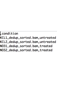
Now let's load the file into our workspace. The commands read.table, read.csv, and read.delim are all related with the exception of different default parameters. They all read a text file and load it into your workspace as a data.frame. Additonally it loads all columns that are character vectors and makes them factors. The first option for all the different versions is the neame of the file. After that, unless you have memorized the options for the commands, explicitly state which parameters you are providing.
expdesign <- read.csv("expdesign.txt", row.names=1, sep=",")
Counting the Reads
Now we will use the GenomicAlignments package to determine where the reads are mapping. Remember we decided to map the sequences to the genome so we can make new discoveries such as novel genes, alternative splicing, and also anti-sense transcripts. In the event that the reference genome is not sequenced, one would have to assemble the RNA-seq reads first to identify all the genes that were detected in the RNA-seq samples. However assembling the transcriptome is quite a complicated process and requires a lot of time and manual curation to produce quality transcripts. We are fortunate that we are using Arabidopsis data whose genome was sequenced in 2000.
The function summarizeOverlaps takes the bam files and the gene annotation to count the number of reads that are matching a gene. The union mode means if a read matches an area where two genes overlap, then it is not counted. We can also provide other parameters such as whether sequence was single-end or pair-end.
library("GenomicAlignments")
## Warning: package 'GenomicAlignments' was built under R version 3.2.3

## Loading required package: SummarizedExperiment

## Warning: package 'SummarizedExperiment' was built under R version 3.2.3
se <- summarizeOverlaps(features=ebg,
                        reads=bamfiles,
                        mode="Union",
                        singleEnd=TRUE,
                        ignore.strand=TRUE )

counts = assay(se)
Filtering the Counts Now, if you remember from the lecture, genes that are expressed at a very low level are extremely unreliable. We will remove all genes if neither of the groups ( KCL or KNO3 ) have a median count of 10 and call the new dataframe counts_filtered.
medianCountByGroup = t(apply(counts, 1, tapply, expdesign, median)) maxMedian=apply(medianCountByGroup, 1, max)
counts_filtered = counts[maxMedian>=10,]
Differentially Expressed Genes
Now that we have the counts table filtered, we can start to determine if any of the genes are significantly differentially expressed using DESeq. DESeq performs a pairwise differential expression test by creating a negative binomial model.
Now we can create an object that DESeq needs using the function newCountDataSet. In order to create this dataset, we need the filtered data frame of read counts and the factor that will help group the data based on the condition.
library(DESeq)
## Warning: package 'DESeq' was built under R version 3.2.3

## Loading required package: locfit

## locfit 1.5-9.1 2013-03-22

##
## Attaching package: 'locfit'

## The following objects are masked from 'package:GenomicAlignments':
##
## left, right

## Loading required package: lattice

## Welcome to 'DESeq'. For improved performance, usability and
## functionality, please consider migrating to 'DESeq2'.
cds = newCountDataSet(counts_filtered, expdesign$condition)
Before the actual test, DESeq has to consider the difference in total reads from the different samples. This is done by using estimateSizeFactors function.
cds = estimateSizeFactors(cds)
Next DESeq will estimate the dispersion ( or variation ) of the data. If there are no replicates, DESeq can manage to create a theoretical dispersion but this is not ideal.
cds = estimateDispersions( cds )
plotDispEsts( cds )
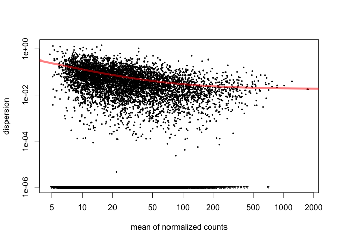
The plot shows us that as the gene's read count increases, dispersion decreases, which is what we expect. Now we will tell DESeq what we would like to compare. Then we will use the adjusted p-value ( p-value corrected for multiple hypothesis testing ) for our cutoff.
res = nbinomTest( cds, "untreated", "treated" )
head(res)
## id baseMean baseMeanA baseMeanB foldChange log2FoldChange
## 1 AT1G01010 21.45700 27.32565 15.58834 0.5704655 -0.8097885
## 2 AT1G01040 44.92871 39.63235 50.22508 1.2672748 0.3417294
## 3 AT1G01050 14.11043 12.85400 15.36686 1.1954923 0.2576048
## 4 AT1G01060 63.99045 71.62446 56.35645 0.7868324 -0.3458717
## 5 AT1G01090 92.24328 80.91875 103.56782 1.2798990 0.3560299
## 6 AT1G01100 180.46426 153.25272 207.67579 1.3551197 0.4384203
## pval padj
## 1 0.1238439 1
## 2 0.3625881 1
## 3 0.7524904 1
## 4 0.4788409 1
## 5 0.2472544 1
## 6 0.1022170 1
sum(res$padj < 0.05, na.rm=T)
## [1] 208
The sum command is normally used to add numberic values. However in logic vectors, TRUE=1 and FALSE=0, so we can use the sum function to count the number of "TRUE" in the vector. In the example we counted the number of genes that have a an adjusted p-value less than 0.05.
MA Plot
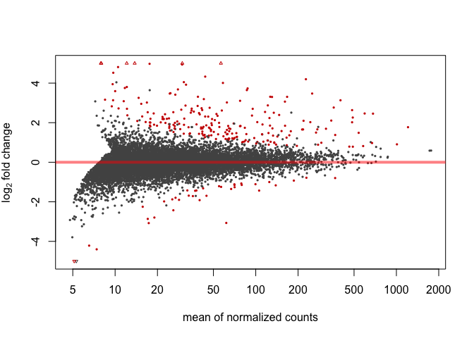
Here's an MA plot that shows as the average count of a gene increases, a smaller fold change is needed for something to be significant. For this reason, it is often helpful to require that the log2foldchange also be greater than or less than negative of some cutoff.
plotMA(res, ylim=c(-5,5))
Significant genes
Let's use the same values for our cutoff to determine which genes we want to consider as significantly differentially expressed. The resSigind variable will contain genes that are induced and resSigrep will contain genes that are repressed when the plants are treated with Nitrate. To create one dataframe of differentially expressed genes, let's combine the two dataframe. We can use the rbind command because the columns are the same in both sets. To show the name of the genes, simply look in the id column of the dataframe.
resSigind = res[ which(res$padj < 0.1 & res$log2FoldChange > 1), ]
resSigrep = res[ which(res$padj < 0.1 & res$log2FoldChange < -1), ]
resSig = rbind(resSigind, resSigrep)

resSigind$id
## [1] "AT1G03850" "AT1G07150" "AT1G08090" "AT1G08100" "AT1G08650"
## [6] "AT1G11655" "AT1G12580" "AT1G13245" "AT1G13300" "AT1G13430"
## [11] "AT1G14340" "AT1G19050" "AT1G21000" "AT1G22170" "AT1G22500"
## [16] "AT1G22650" "AT1G23310" "AT1G23870" "AT1G24280" "AT1G25550"
## [21] "AT1G30510" "AT1G30840" "AT1G31770" "AT1G32380" "AT1G32920"
## [26] "AT1G35560" "AT1G43710" "AT1G45249" "AT1G49000" "AT1G49160"
## [31] "AT1G49450" "AT1G49860" "AT1G50110" "AT1G55120" "AT1G58410"
## [36] "AT1G59960" "AT1G59970" "AT1G60710" "AT1G61740" "AT1G62180"
## [41] "AT1G63940" "AT1G64190" "AT1G66140" "AT1G67110" "AT1G67920"
## [46] "AT1G68238" "AT1G68670" "AT1G68880" "AT1G70260" "AT1G70410"
## [51] "AT1G73920" "AT1G74030" "AT1G77760" "AT1G78000" "AT1G78050"
## [56] "AT1G80310" "AT1G80380" "AT1G80440" "AT2G15620" "AT2G16060"
## [61] "AT2G17820" "AT2G26820" "AT2G26980" "AT2G27510" "AT2G27830"
## [66] "AT2G28550" "AT2G28780" "AT2G28890" "AT2G30040" "AT2G30100"
## [71] "AT2G30660" "AT2G30670" "AT2G33550" "AT2G36320" "AT2G36580"
## [76] "AT2G41310" "AT2G41440" "AT2G41560" "AT2G41660" "AT2G43760"
## [81] "AT2G46620" "AT2G47160" "AT2G48080" "AT3G04530" "AT3G05200"
## [86] "AT3G07350" "AT3G10520" "AT3G11410" "AT3G13560" "AT3G13730"
## [91] "AT3G14260" "AT3G16560" "AT3G17510" "AT3G17609" "AT3G18560"
## [96] "AT3G19030" "AT3G22550" "AT3G22850" "AT3G25790" "AT3G28690"
## [101] "AT3G29034" "AT3G46640" "AT3G47520" "AT3G47980" "AT3G48360"
## [106] "AT3G49940" "AT3G52360" "AT3G52960" "AT3G55980" "AT3G57520"
## [111] "AT3G58610" "AT3G58760" "AT3G60330" "AT3G60750" "AT3G61880"
## [116] "AT3G63110" "AT4G00416" "AT4G00630" "AT4G02380" "AT4G02920"
## [121] "AT4G04610" "AT4G04745" "AT4G05070" "AT4G05390" "AT4G09620"
## [126] "AT4G13890" "AT4G15340" "AT4G17550" "AT4G18340" "AT4G21350"
## [131] "AT4G24620" "AT4G24670" "AT4G25835" "AT4G26130" "AT4G26970"
## [136] "AT4G29740" "AT4G29905" "AT4G31730" "AT4G31910" "AT4G32950"
## [141] "AT4G34000" "AT4G34419" "AT4G34740" "AT4G34750" "AT4G34800"
## [146] "AT4G34860" "AT4G35260" "AT4G36010" "AT4G36040" "AT4G37540"
## [151] "AT4G37610" "AT5G01340" "AT5G03330" "AT5G03380" "AT5G04840"
## [156] "AT5G05250" "AT5G06570" "AT5G07890" "AT5G09800" "AT5G09850"
## [161] "AT5G10030" "AT5G10210" "AT5G12470" "AT5G12860" "AT5G13110"
## [166] "AT5G13420" "AT5G14060" "AT5G14690" "AT5G14760" "AT5G18840"
## [171] "AT5G19120" "AT5G19260" "AT5G19970" "AT5G20540" "AT5G20885"
## [176] "AT5G26010" "AT5G27100" "AT5G35620" "AT5G35630" "AT5G39590"
## [181] "AT5G40850" "AT5G41670" "AT5G42830" "AT5G47100" "AT5G47560"
## [186] "AT5G47740" "AT5G49480" "AT5G50200" "AT5G51440" "AT5G51830"
## [191] "AT5G52050" "AT5G53460" "AT5G54130" "AT5G54170" "AT5G56080"
## [196] "AT5G58320" "AT5G58700" "AT5G58900" "AT5G63160" "AT5G65030"
## [201] "AT5G65210" "AT5G65980" "AT5G66530" "AT5G67420"
resSigrep$id
## [1] "AT1G13110" "AT1G27030" "AT1G29050" "AT1G55760" "AT1G64590"
## [6] "AT1G67810" "AT1G69850" "AT1G76350" "AT1G79320" "AT2G17710"
## [11] "AT2G32560" "AT2G36910" "AT3G01290" "AT3G09220" "AT3G13620"
## [16] "AT3G21420" "AT3G44540" "AT4G08300" "AT4G12290" "AT4G17030"
## [21] "AT4G17670" "AT4G25970" "AT4G28350" "AT4G35720" "AT5G03760"
## [26] "AT5G06510" "AT5G10770" "AT5G16570" "AT5G18130" "AT5G19140"
## [31] "AT5G40780" "AT5G41610" "AT5G64410"
Gene Annotations
Great ! We have genes that are differentially expressed, what do we know about these genes ? The gene identifier we obtained from the GTF file is referred to as TAIR identifiers (a consortium that used to release Arabidopsis genome annotations) I managed to download the gene description for all the genes. Let's load them into the workspace and find out what are the names of the genes.Since the set of repressed genes is smaller, let's see what we can find out about them.
Before we do this, note that the identified in the gene_description file is slightly different ( the file contains the transcript identifier that ends with "." and a number), Let's replace every occurrence of . and a number with nothing. Then we will be able to use match to find where our gene is in the description file so we can only print out that row.
gene_description <- read.delim("gene_description_20131231.txt",
header=FALSE, quote="")
genenames = gsub("[.][1234567890]", "",
gene_description[,1])

gene_description[,1]=genenames

gene_match_rows=match(resSigrep$id, gene_description[,1])
gene_description[gene_match_rows,c(1,3)]
## V1
## 3100 AT1G13110
## 21972 AT1G27030
## 2839 AT1G29050
## 1972 AT1G55760
## 1820 AT1G64590
## 22251 AT1G67810
## 20881 AT1G69850
## 1304 AT1G76350
## 22196 AT1G79320
## 22685 AT2G17710
## 6908 AT2G32560
## 6574 AT2G36910
## 26917 AT3G01290
## 9196 AT3G09220
## 9713 AT3G13620
## 10123 AT3G21420
## 8077 AT3G44540
## 14581 AT4G08300
## 15339 AT4G12290
## 14362 AT4G17030
## 14147 AT4G17670
## 24600 AT4G25970
## 13187 AT4G28350
## 13966 AT4G35720
## 25150 AT5G03760
## 15855 AT5G06510
## 20396 AT5G10770
## 27313 AT5G16570
## 19087 AT5G18130
## 20217 AT5G19140
## 17046 AT5G40780
## 17702 AT5G41610
## 19209 AT5G64410
## V3
## 3100 cytochrome P450, family 71 subfamily B, polypeptide 7
## 21972
## 2839 TRICHOME BIREFRINGENCE-LIKE 38
## 1972 BTB/POZ domain-containing protein
## 1820 NAD(P)-binding Rossmann-fold superfamily protein
## 22251 sulfur E2
## 20881 nitrate transporter 1:2
## 1304 Plant regulator RWP-RK family protein
## 22196 metacaspase 6
## 22685
## 6908 F-box family protein
## 6574 ATP binding cassette subfamily B1
## 26917 SPFH/Band 7/PHB domain-containing membrane-associated protein family
## 9196 laccase 7
## 9713 Amino acid permease family protein
## 10123 2-oxoglutarate (2OG) and Fe(II)-dependent oxygenase superfamily protein
## 8077 fatty acid reductase 4
## 14581 nodulin MtN21 /EamA-like transporter family protein
## 15339 Copper amine oxidase family protein
## 14362 expansin-like B1
## 14147 Protein of unknown function (DUF581)
## 24600 phosphatidylserine decarboxylase 3
## 13187 Concanavalin A-like lectin protein kinase family protein
## 13966 Arabidopsis protein of unknown function (DUF241)
## 25150 Nucleotide-diphospho-sugar transferases superfamily protein
## 15855 nuclear factor Y, subunit A10
## 20396 Eukaryotic aspartyl protease family protein
## 27313 glutamine synthetase 1;4
## 19087
## 20217 Aluminium induced protein with YGL and LRDR motifs
## 17046 lysine histidine transporter 1
## 17702 cation/H+ exchanger 18
## 19209 oligopeptide transporter 4